Visualize Probability Distributions • vistributions

Visualize probability distributions

vistributions visualizes the normal, t, F, chi-square and binomial distributions with ggplot2. Each family exposes the same grammar: _plot for the shape, _perc for quantiles from probabilities and _prob for probabilities from quantiles, with shaded tails and annotated cutoffs for teaching and publication.

Installation

# Install release version from CRAN
install.packages("vistributions")

# Install development version from GitHub
# install.packages("devtools")
devtools::install_github("rsquaredacademy/vistributions")

Supported distributions

Family	Shape	Quantile from p	Probability from q
Normal	`vdist_normal_plot()`	`vdist_normal_perc()`	`vdist_normal_prob()`
t	`vdist_t_plot()`	`vdist_t_perc()`	`vdist_t_prob()`
F	`vdist_f_plot()`	`vdist_f_perc()`	`vdist_f_prob()`
Chi-square	`vdist_chisquare_plot()`	`vdist_chisquare_perc()`	`vdist_chisquare_prob()`
Binomial	`vdist_binom_plot()`	`vdist_binom_perc()`	`vdist_binom_prob()`

All plotting functions print by default and return the ggplot object invisibly. Pass print_plot = FALSE to get a composable plot object for further customization with + labs(), + theme_minimal() or ggplot2::ggsave().

Articles

Explore Distributions

Usage

Normal distribution

# distribution shape
vdist_normal_plot()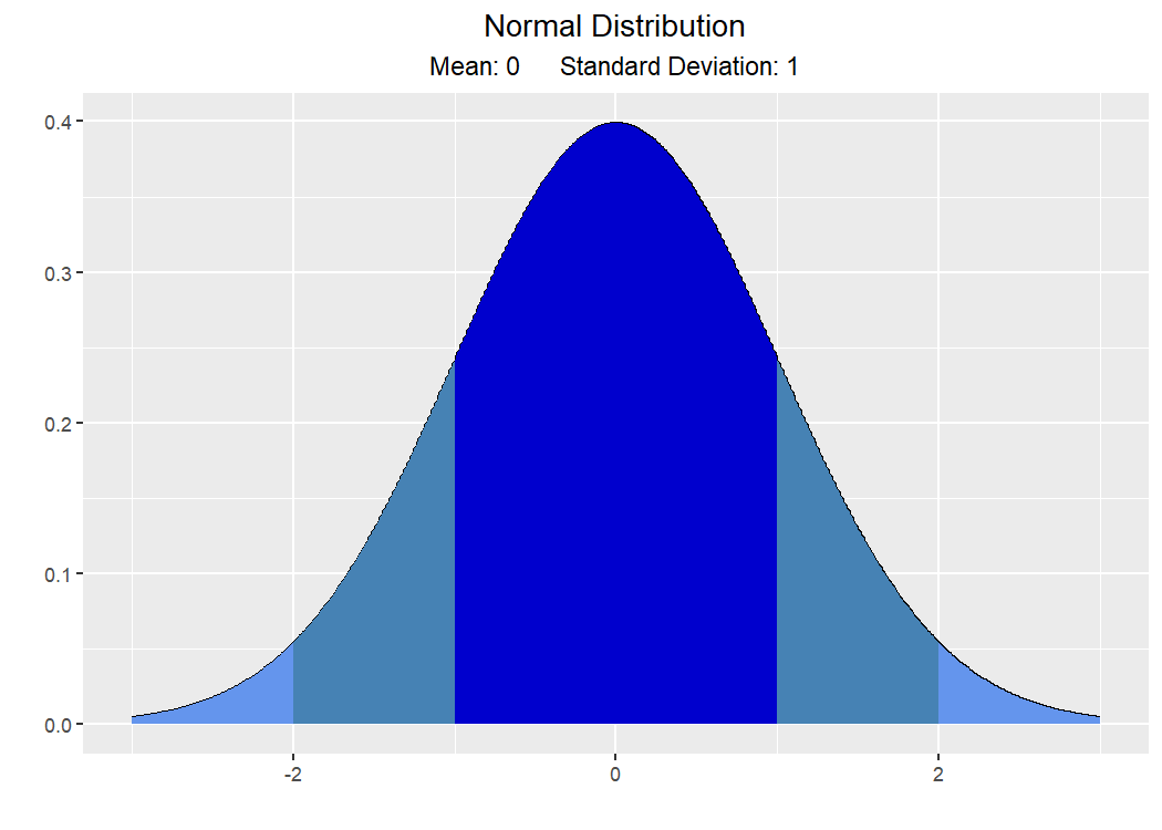


# quantile from a probability (upper 10%)
vdist_normal_perc(0.10, mean = 60, sd = 3, type = "upper")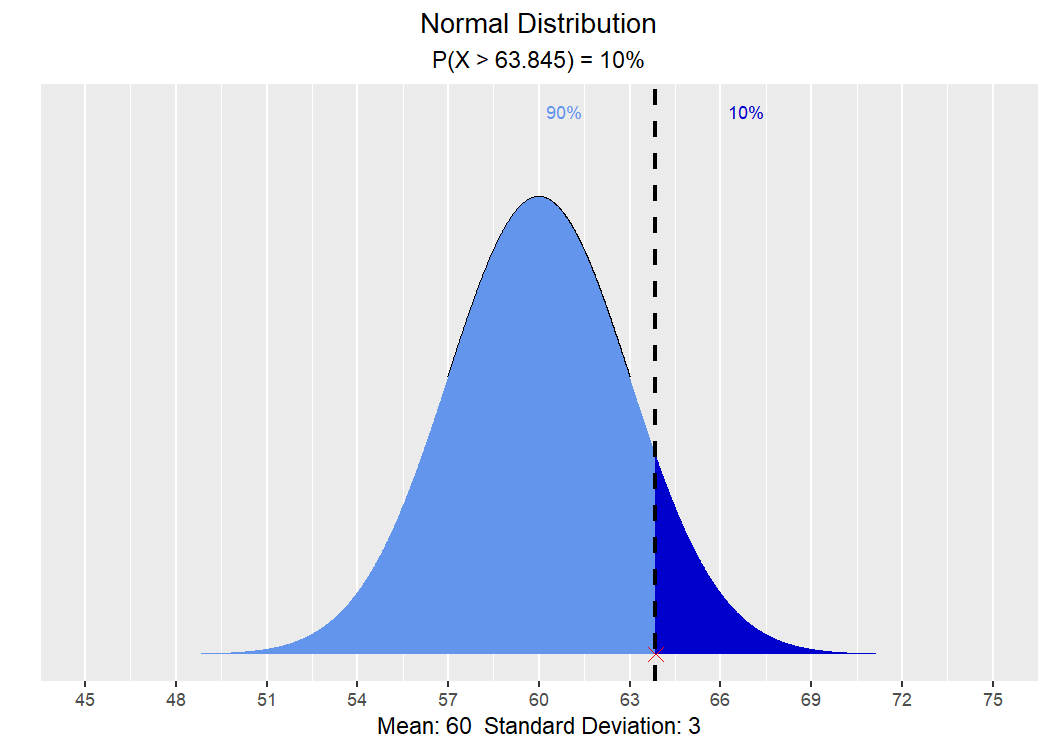


# probability from quantiles (middle 50%)
vdist_normal_prob(c(85, 100), mean = 90, sd = 4, type = "both")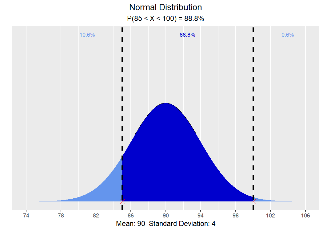

t distribution

vdist_t_plot(df = 8)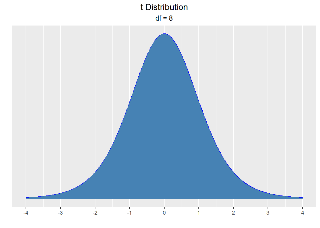


# upper 15th percentile
vdist_t_perc(0.15, df = 8, type = "upper")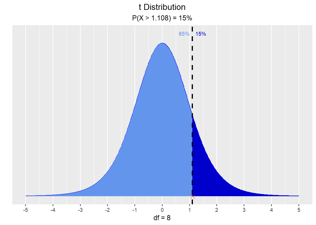


# probability between -2 and 2
vdist_t_prob(2, df = 6, type = "interval")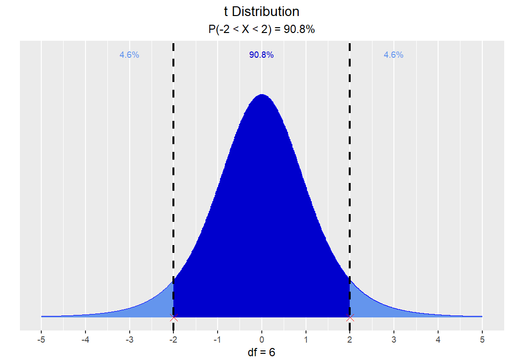

Chi-square distribution

vdist_chisquare_plot(df = 5)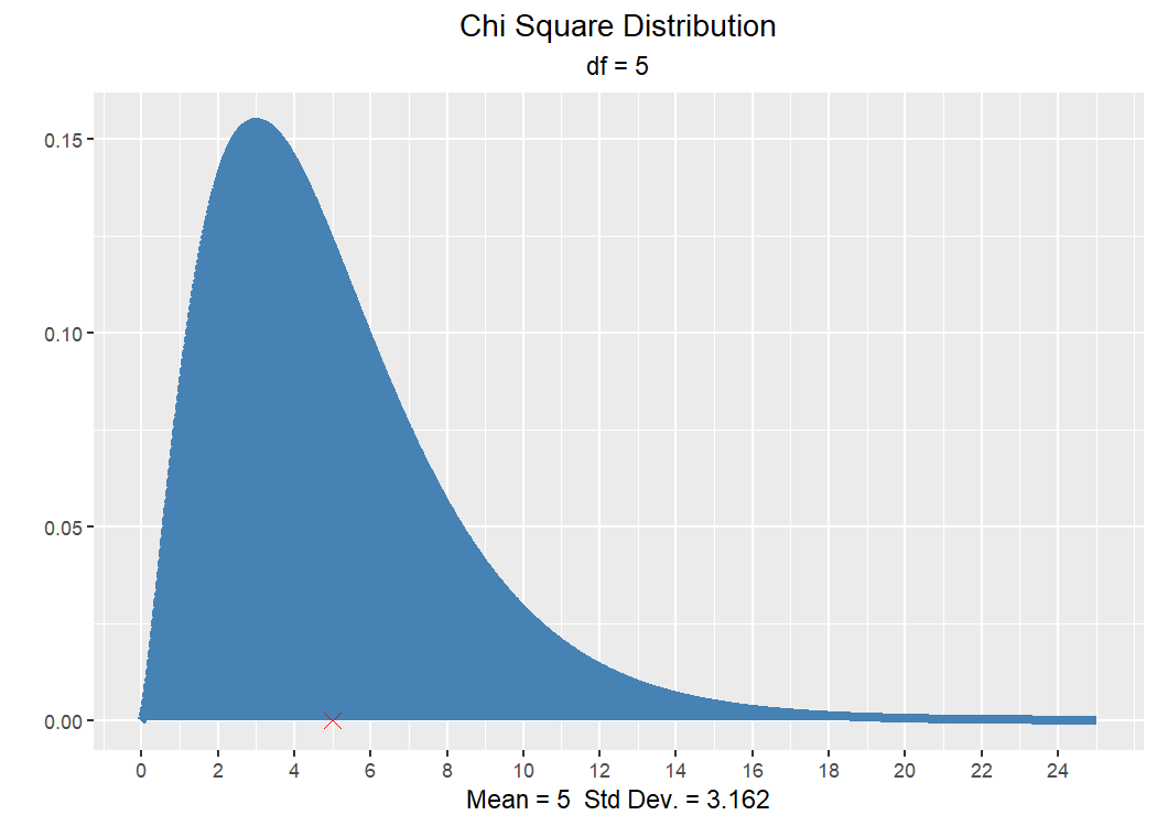


# tenth percentile
vdist_chisquare_perc(0.10, df = 8, type = "lower")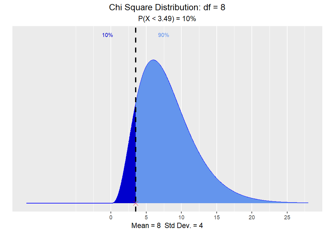


# P(X > 8.79) with 12 df
vdist_chisquare_prob(8.79, df = 12, type = "upper")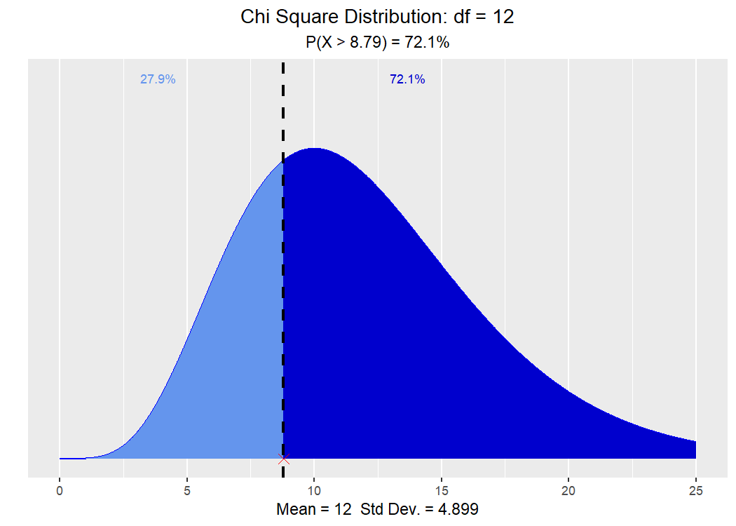

F distribution

vdist_f_plot()


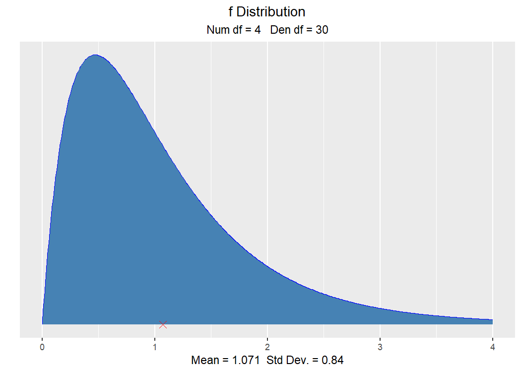
# upper twentieth percentile, F(4, 5)
vdist_f_perc(0.20, num_df = 4, den_df = 5, type = "upper")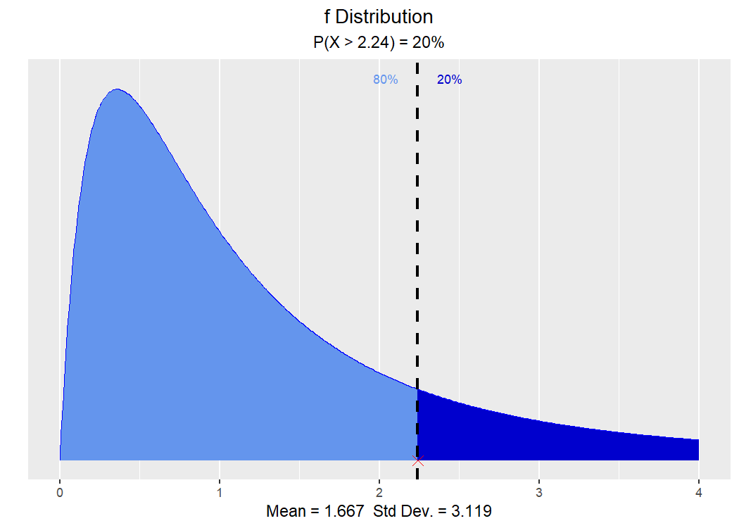


# P(X > 3.89), F(4, 5)
vdist_f_prob(3.89, num_df = 4, den_df = 5, type = "upper")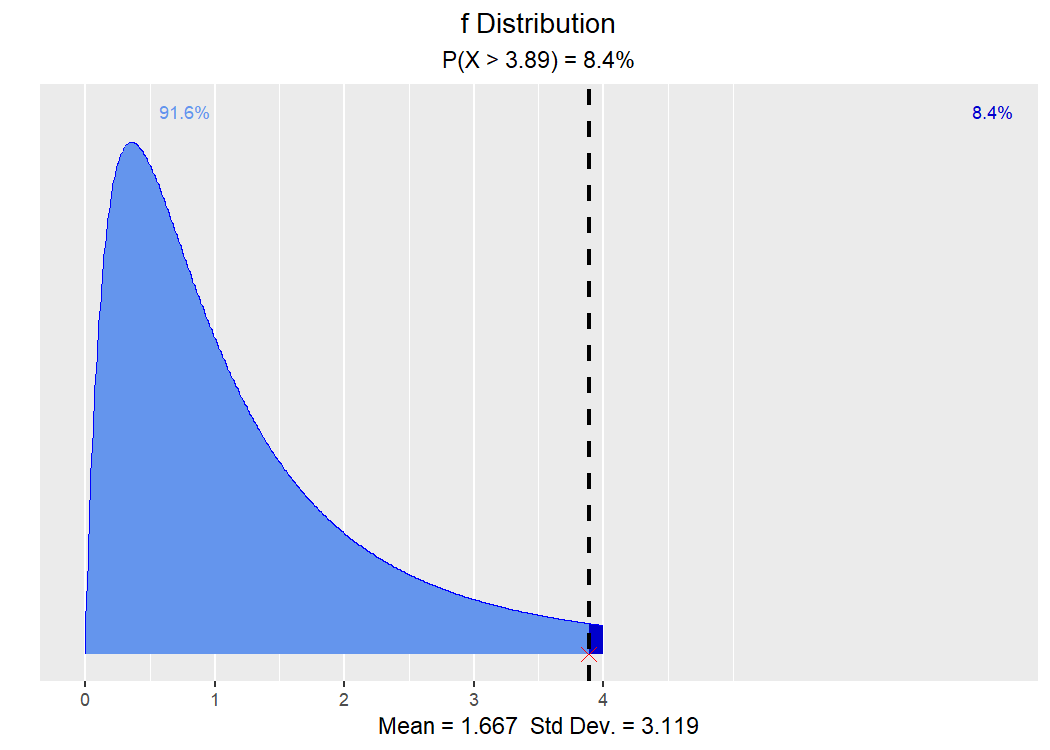

Binomial distribution

vdist_binom_plot(12, 0.2)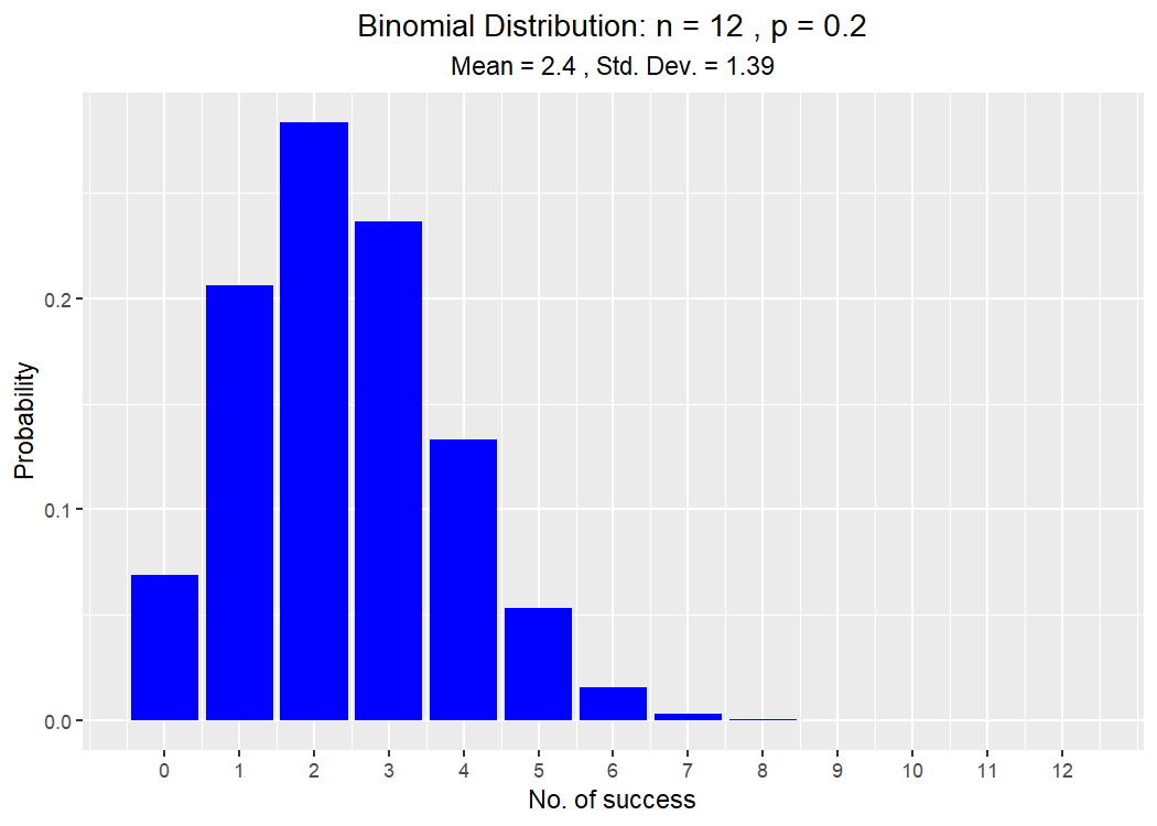


# exactly 4 successes out of 12
vdist_binom_prob(12, 0.2, 4, type = "exact")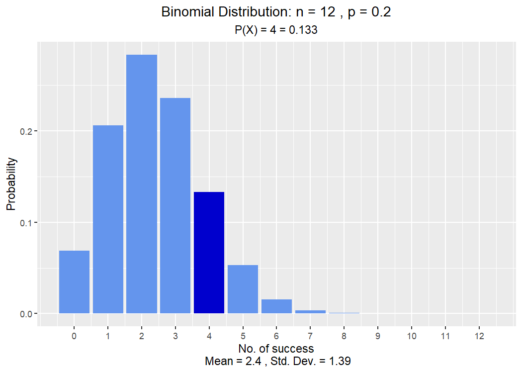


# at most 1 success
vdist_binom_prob(12, 0.2, 1, type = "lower")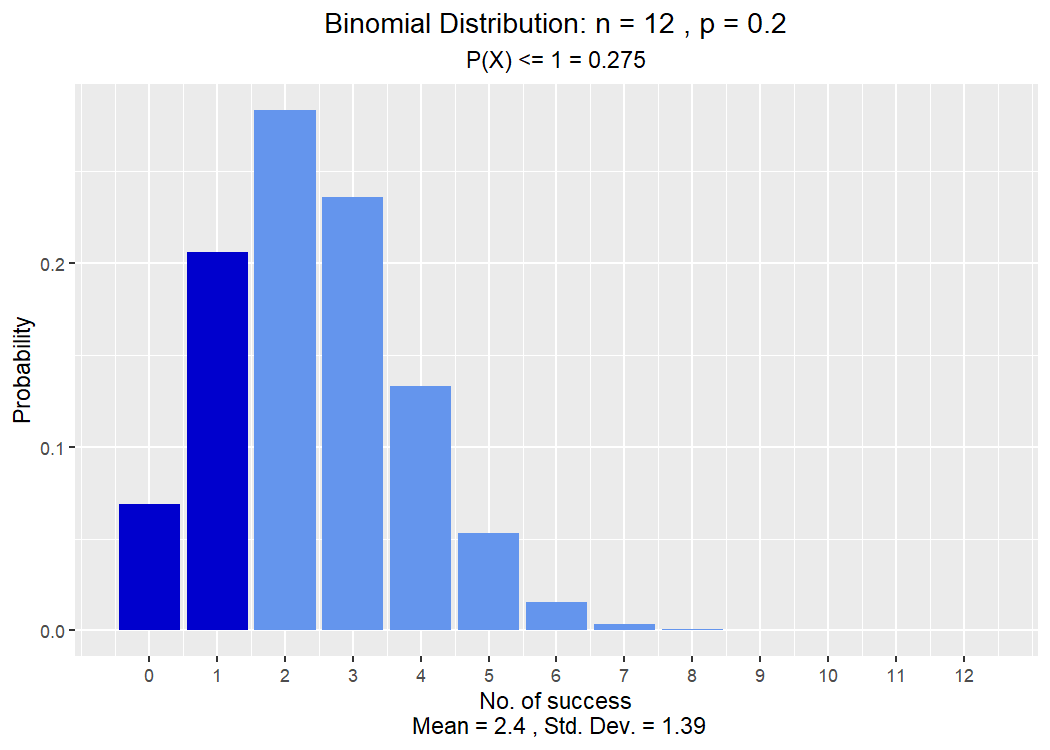

Customize the plot object

library(ggplot2)

p <- vdist_normal_plot(mean = 60, sd = 3, print_plot = FALSE)
p + theme_minimal() + labs(title = "Normal(60, 3)")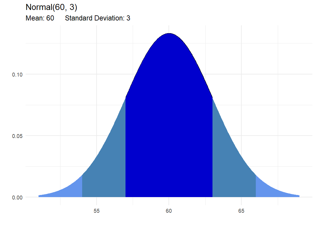

How it compares

visualize covers more families with base graphics; vistributions focuses on five teaching families with annotated ggplot2 output.
mosaic (xpnorm() and friends) is course-framework bound; vistributions works standalone.
distributional + ggdist is the modeling-grade stack; vistributions is the lightweight classroom companion. Native distributional dispatch is planned for v1.0 (see roadmap/).

Getting Help

If you encounter a bug, please file a minimal reproducible example using reprex on GitHub. For questions and clarifications, use StackOverflow.